Reflection Week 5

This week in AP Biology, we focused primarily on the basics of Molecular Biology so we have a level to learn more complicated things from. We started off the week with a video from the weird world series to dismiss a few of the Monday blues. On Tuesday, we covered a few labs and video worksheets in which we answered the basics of biochemistry. On Thursday, the hardest day in my opinion, we did a lab where we matched molecular structures to their groups and names.

On Tuesday, we discussed the 4 different types of major macromolecules.

1. Lipids include fats and waxes – they consist of one monomer and they store energy.
2. Nucleic Acids (ex. DNA, RNA) nucleotide monomers, made of adenine, thymine, guanine, cytosine, and uracil.
3. Proteins (ex. collagen, hemoglobin) amino acid monomers
4. Carbohydrates (ex. glucose, sucrose) supply energy, sugars

The types of molecules can be more broadly categorized into:

1. Monomer: Molecules that can be bonded to other monomers, “building blocks of life”
2. Polymer: A large molecule or macromolecule composed of repeated subunits

On Thursday, we focused on how to take these molecular properties and use them to divide different macromolecules into groups. These could have been subcategories such as nucleotides, ribose and fatty acids. This lab was incredibly hard for me to mentally wrap my head around it, and I’m still working on it as we speak. Carbon, hydrogen and oxygen make up all parts of molecules, but sometimes nitrogen, sulfur and phosphorus are also present. In amino acids, the molecules are focused around a central carbon backbone and has a double bond with oxygen. Steroids, or cholesterol,  have multiple rings of carbon atoms and the carbon sits invisibly at every angle in the diagram. For this reason the beehive-shaped m=diagrams were usually distinguished as steroids. Fatty acids are the long chained diagrams and are a type of lipid. They’re made of hydrocarbon chains with a carboxyl group at one end. In carbohydrates there is about a 1:1 ratio of oxygen to hydrogen and these sugars can be divided into monosaccharides, disaccharides, and straight chain sugars. With the nucleic acids we observed simple and complex nitrogenous bases. These molecules can have nitrogen in them.

This week was difficult for me to understand since I didn’t have a very good experience with chemistry class, but I really want to learn and improve my knowledge of it. This topic delves into the science behind big idea 2, and the building blocks behind all living organisms. This is to ensure that we grasp the basics, so we can use the knowledge to understand more complicated topics.

In the future, I would love to understand more about how different structures are formed in polymers and how I can identify one macromolecule and differentiate it to others.

Sources:

Sciencing: 4 Macromolecules of Life

Macromolecules for Identification

 

Week 4 Reflective Response

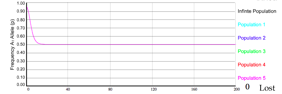
This week in AP Biology, we started with a brand new lab involving investigating microevolution by using a population generation program. Through this lab we disturbed each of the 5 standards of Hardy Weinberg equilibrium in order to see how the population evolves in response. I decided to experiment with the heterozygote advantage within a population, which revealed their dominant and recessive allelic equilibrium. This lab is using a quantifying manner to approach Big Idea #1 by using our knowledge of the 5 standards of Hardy Weinberg equilibrium to experiment and visualize what is happening within the population.

In class, we discussed 2 new major ideas: speciation and classification. A species is a population whose members can interbreed and produce viable and fertile offspring. Speciation is created by a series of evolutionary processes that result in the reproductive isolation of a population. Darwin called it the “mystery of mysteries”. There are two types of speciation: Allopatric and Sympatric.

Allopatric is a population isolated due to physical barriers. An example of this would be when the Grand Canyon formed, it separated one species of squirrel. The squirrels evolved on their side and now no longer recognize one another as a mate. An example of allopatric speciation is the separation of marine creatures on either side of Central America when the Isthmus of Panama closed about 3 million years ago, creating a land bridge between North and South America. Nancy Knowlton of the Smithsonian Tropical Research Institute in Panama has been studying this geological event and its effects on populations of snapping shrimp. She and her colleagues found that shrimp on one side of the isthmus appeared almost identical to those on the other side — having once been members of the same population.

On the other hand, sympatric speciation is when a species remains in the same physical area but become reproductively isolated from one another. For example, gene flow from one part of the population of flies stops from the other when they choose to lay their eggs in different locations. These are all ways a species can be isolated from one another genetically (isolationism). However, there can also be a hybrid population which is caused by gene flow between two species. A real life example of this would be when 200 years ago, the ancestors of apple maggot flies laid their eggs only on hawthorns — but today, these flies lay eggs on hawthorns (which are native to America) and domestic apples (which were introduced to America by immigrants and bred). Females generally choose to lay their eggs on the type of fruit they grew up in, and males tend to look for mates on the type of fruit they grew up in. So hawthorn flies generally end up mating with other hawthorn flies and apple flies generally end up mating with other apple flies. This means that gene flow between parts of the population that mate on different types of fruit is reduced.

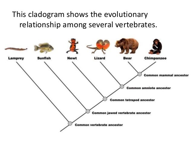
Secondly, we learned how to classify species using the old school method and the new school method. The old school method was created by Carl Linnaeus based off of the hierarchy of life. This was based on domain and kingdom. There were three domains: Bacteria, Eukarya, and Archaea and five kingdoms: Monera, Protista, Fungi, Plantae, and Animalia. This system proved to be inefficient because there were too many different species that were interrelated to one another and this discounted everything we could not see (microscopic) as one species. The new school method was used DNA to find relativity to other animals. We could now look deeper than the surface value of physical appearance and see the genetic code of the species by using cladograms (which show us how they evolved from one common ancestor).

To create a cladogram, you must:

1. Determine how many species have a particular characteristic in common
2. Group the species so that the most number of species have the most characteristics in common
3. Apply the rules of maximum parsimony and likelihood
4. Sort the types of groups within a cladogram into monophyletic (all descendants of 1 common ancestor), paraphyletic (some he descendants have 1 common ancestor), or polyphyletic.

This big idea showed us how exactly species evolve, and from who/what original ancestors. I would love to explore further spectrums of speciation and classification by being able to sort our own species and classify them in a program or “game”.

Websites

Sympatric Speciation

Allopatric Speciation – PBS

Week 3 Reflective Response

This week, we learned about the Hardy-Weinberg equation and relating theory. It hypothetically introduces a non-evolving population that preserves allele frequencies in order to serve as a model for comparison. In nature, populations can never be in Hardy-Weinberg equilibrium because of 5 things:

1. There can be no genetic mutations in the DNA – it would create genetic diversity
2. No sexual selection, only random selection – otherwise a certain trait will be favored in an environment
3. No genetic drift – environmental changes can lead to division of population
4. No migration – can’t be influenced by other environments that could stimulate new traits
5. No competition – predators won’t kill one trait off, so new traits develop

The Hardy-Weinberg equation is p+q=1 for allele frequencies and p^2+2pq+q^2=1 is for genotype frequencies. The p stands for the dominant allele, or p^2 homozygous dominant. The q stands for recessive allele, or q^2 for homozygous recessive. The 2pq stands for the heterozygous representation. The recessive allele (q) is what creates a defective protein, vs. the dominant allele (p) making regular proteins. In order to solve this equation in an example problem, here is what you do:

• In a population, the dominant phenotype of a certain trait occurs 91% of the time. What is the frequency of the dominant allele?

Since the dominant phenotype shows up in both heterozygous and homozygous dominant genotypes, you subtract .91 from 1. This will give you .09, which is the recessive genotype (q^2). Next, find the square root (.03) which is the recessive allele frequency (q). Take this value away from 1 because p+q=1. You get 7 – square 7 (.49) to find the homozygous dominant genotype frequency (p^2). Then you can take the original values to plus in to 2pq to find the heterozygous genotype frequency (.42). Now that you have all the data, you can determine that the dominant allele frequency is .7 or 7%.

Putting this theory in practice, during class we did a collective lab in which we imitated mating within a population. We attempted creating an ideal Hardy-Weinberg population,  selecting against homozygous recessive, examining the heterozygous advantage and genetic drift in populations. Although our results were similar to what we expected, they weren’t perfect because we aren’t an unlimited population like in nature. Through this, we also realized that it is naturally impossible to achieve all of the five conditions to make a Hardy-Weinberg population.

To conclude, this week we took our knowledge of big idea #1 and learned how to measure it and sort data from it. Although it wasn’t necessarily 100% correct, it still communicated the main ideas of population genetics. I would love to learn about more ways to sort biological data and calculate it through other equations because once I understood how to use the Hardy Weinberg formula, it was fun to use!

Websites:

Hardy Weinberg Formulas – KSU

The Heterozygote Advantage

The Ideal Population